
The most complete way to visualize the results is to bring up the main graphical user interface. Therefore, please type
cal -> gui
The window drawn below (click on it to enlarge it) should appear. On some computers IDL has some difficulty to figure out which color model should be used. If you do not see colours (the red colour only appears after the threshold has been adjusted) please try
cal -> gui,/tru
This will use 24bit colors and might help. In some cases it was useful to close the gui and restart it again. All the modifications are recorded and thus available afterwards.
The graphical user interface is divided into various areas and subpanels. Some of them are interactive.
With exception of the "LAMBDA GUI", all items in the menu bar are also accessible via buttons/areas within the panel itself.
Below the menu bar all used files are listed. These informations can be obtained with the commands
fringefile = cal->get_filename()
photfiles = cal->get_filename(/PHOT)
maskfile = cal->get_filename(/MASK)
where photfiles is an array. The name of the object can be stored in the variable object with the command
object = cal -> get_objectname()
This panel diplays the optical path difference (OPD) vs. the frame number. Clearly visible are the 80µm scans. During each of the 300 scans 40 exposures have been taken leading to a total amount of 12000 frames. After 2000 frames = 50 scans zero OPD has been found at 11.37 mm and MIDI tracked on it with exception of a few scans between frame number 2000 and frame number 5500.
This panel displays the measured flux vs. the frame number. To get the photometry vs. the pixel number type
spec = cal->get_photometry()
print,spec
Default is to return the sum of all 4 spectra. The Keywords /Atotal and /Btotal return the sum of the two (I1 & I2) A- or B-spectra, respectively. Keywords /A1, /A2, /B1, and /B2 return the corresponding spectrum. Everything is in ADU/sec (conversion factor for MIDI: 145 photons/ADU). The command
lambda = cal->lambda()
returns an array that gives wavelength in µm as function of the pixel number. With
cal->set_lambda,lambda
the user can set a wavelength calibration.
This panel displays the flux difference (I1-I2) vs. the frame number, i.e. the modulation in the correlated flux. Before MIDI reached zero OPD no fringes are visible. Afterwards, a strong signal could be detected. By typing
cf = cal->correlflux()
one gets the correlated flux as function of wavelength. This is a 3 by N array, where N is the number of bins in lambda. The first row (cf[0,*]) is the wavelength in the center of the bins, the second row (cf[1,*]) is the width of the wavelength bins, and the third row (cf[2,*]) is the correlated flux in ADU/sec (conversion factor for MIDI: 145 photons/ADU).
Keyword /PLOT will plot the good and bad fringes in the lambda bins, and the correlated flux. Keyword /CFPLOT will plot only the correlated flux.
To set the binning in wavelength one can use the command
cal->set_lambda_bins, start, end, step, width
where start is the number of the first column used, end the number of the last column used, step the spacing between columns, and width the number of columns added for one bin. For example
cal->set_lambda_bins, 0, 100, 25, 50
will set the bins 0...49, 25...74, 50...99, 75...124, and 100...149 pixels. Note that the last bin can extend beyond the given end column. An interactive tool to define the bins is the "LAMBDA GUI". It can be started from the menu or with

This panel displays the maximum amplitude of the fringes in the white light, i.e. integrated over wavelength vs. the scan number. To get the amplitude, we integrate over wavelength, Fourier-transform each scan, add up the power spectrum at the frequencies where we expect fringes, and calculate the square root. To get the maximum amplitude of the white light fringe use
whitelight = cal->whitefringeampl()
The command
fringes = cal->fringes()
returns a 3D-array: fringes[0,*,*] is the OPD and fringes[1,*,*] the fringe amplitude. The third index counts the scan, the second the frame-number within a scan.
 On the lower right panel two histograms are drawn. One displays
the distribution of the scans with respect to the fourier amplitude
and the other with respect to the mean optical path difference. Three
thresholds can be set.
On the lower right panel two histograms are drawn. One displays
the distribution of the scans with respect to the fourier amplitude
and the other with respect to the mean optical path difference. Three
thresholds can be set.
cal->set_thresholds, good, bad, noiseopd
where noiseopd is optional. To read out the current values type
th = cal->get_thresholds()
The percentage of good and bad scans with the current thresholds is returned by
gb = cal->get_percent_goodbad()

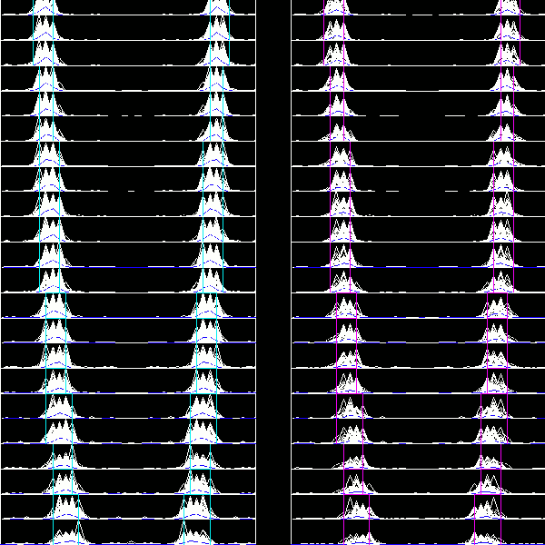
The spectral power of the good and the bad fringes vs. the frequency is plotted on the lower left panel of the GUI. The vertical dashed lines mark the frequency range where fringes are expected, i.e.
ν_min = floor (δ / λ_max + 0.5)
ν_max = floor (δ / λ_min + 0.5)
δ is the length of a scan. The symmetry of the plots, i.e. the right side is a mirrored left side, is an artifact of the fourier transformation. The blue curve is the mean of all the white curves.

By clicking on the plots a new window opens. It displays the plots for the different wavelength bins set with the "lambda gui" or the corresponding command set_lambda_bins (see above). The good fringes are plotted on the left side, the bad fringes on the right side. The frequency range, where the fringes are expected moves from lower to higher frequencies, because the binned wavelengths are decreasing. Another window opens simultaneously, showing the (raw) visibility of the object.
The corresponding command that delivers the same informations is
visi = cal->visibility()
This command is similar to correlflux(), except that visi[2,*] contains the visibility and not the correlated flux. The first row (visi[0,*]) is the wavelength in the center of the bins and the second row (visi[1,*]) is the width of the wavelength bins.
The optional keyword /PLOT plots the above shown lambda-binned spectral power and /VISPLOT the visibility graph.
The panel in the center summarizes the most important quantities given in various subpanels and offers a few buttons.

cal->hardcopy, filename
where filename is the name of
the postscript-file to print to. If the name is omitted it will be
created from the name of the fringe data.
/NCOLOR prints in black and white,
/TRACES prints the traces, too, and
/DONTCLOSE doesn't close the file
afterwards, so you can append more plots
obj_destroy, cal
If you fail to do this and re-use the variable, the object
will stay in memory. There's no way to destroy it and free the
memory once the reference to it is lost (IDL has no garbage
collection).
Fringe Movie Fourier Movie 

Previous: XMDV
Next: Visibilities